Fred Park
  • Home
  • Research
  • Teaching
  • Resources
  • Personal
  • Blog

Image Denoising

5/2/2016

4 Comments

 
In our Pi Mu Epsilon Talk last week, Dr. Weisbart talked about the noise process and how noise manifests itself in images. Here I say a few words about the image denoising process, i.e. noise removal. Given a grayscale image $f:[0,1]\times[0,1]\rightarrow [0,255]$ where $f(x,y)=0$ denotes black and $f(x,y)=255$ denotes white; any value in between is a shade of gray. Color images are the extension where a pixel location $(x,y)$ maps to a vector $[R,G,B]$. Each component $R$, $G$, and $B$ are grayscale images themselves representing the red, green, and blue channels respectively. In the talk last week, the speaker spoke about Poisson noise processes. In general, since such noise processes can be approximated by Gaussian noise via the Central Limit Theorem, we assume an additive Gaussian noise from a modeling perspective. i.e. if $u_c$ denotes the clean image, then the image $f$ degraded by noise is modeled as the following:
$$f(x,y) =  u_c(x,y) + \eta(x,y)$$
where $\eta(x,y)$ is a random variable from a Gaussian distribution of mean zero and standard deviation $\sigma$. Thus, the image denoising problem is the inverse problem of finding $u_c$ given the noisy image $f$ and some statistics on the noise.

One of the most celebrated and utilized image denoising models is the TV-Denoising Model from Rudin, Osher, and Fatemi. The model is in a functional minimization form:
$$\min_{u} \left\{ J[u] =  \frac{1}{2}\int_{\Omega} (f-u)^2\,dx + \lambda \int_{\Omega} |\nabla u| \right\}$$
where $\Omega$ is the image domain (rectangle) and the Total variation semi-norm $\int |\nabla u|$ is defined in the distributional sense:
$$TV(u) = \int_{\Omega}|\nabla u| = \sup \left\{\int_{\Omega} u(x) \xi(x) \, dx \, | \, \xi \in C_c^1(\Omega, \mathbf{R}^n), \ \|\xi\|_{\infty} \leq 1\right\}.$$ 
The model is a balance between data fitting and regularity where the parameter $\lambda$ controls this tradeoff.

There are numerous ways to minimize the above TV model but one of the simplest is via gradient descent:
$$u_ t = -\nabla J[u] = f-u + \nabla \cdot \frac{\nabla u}{|\nabla u|}$$
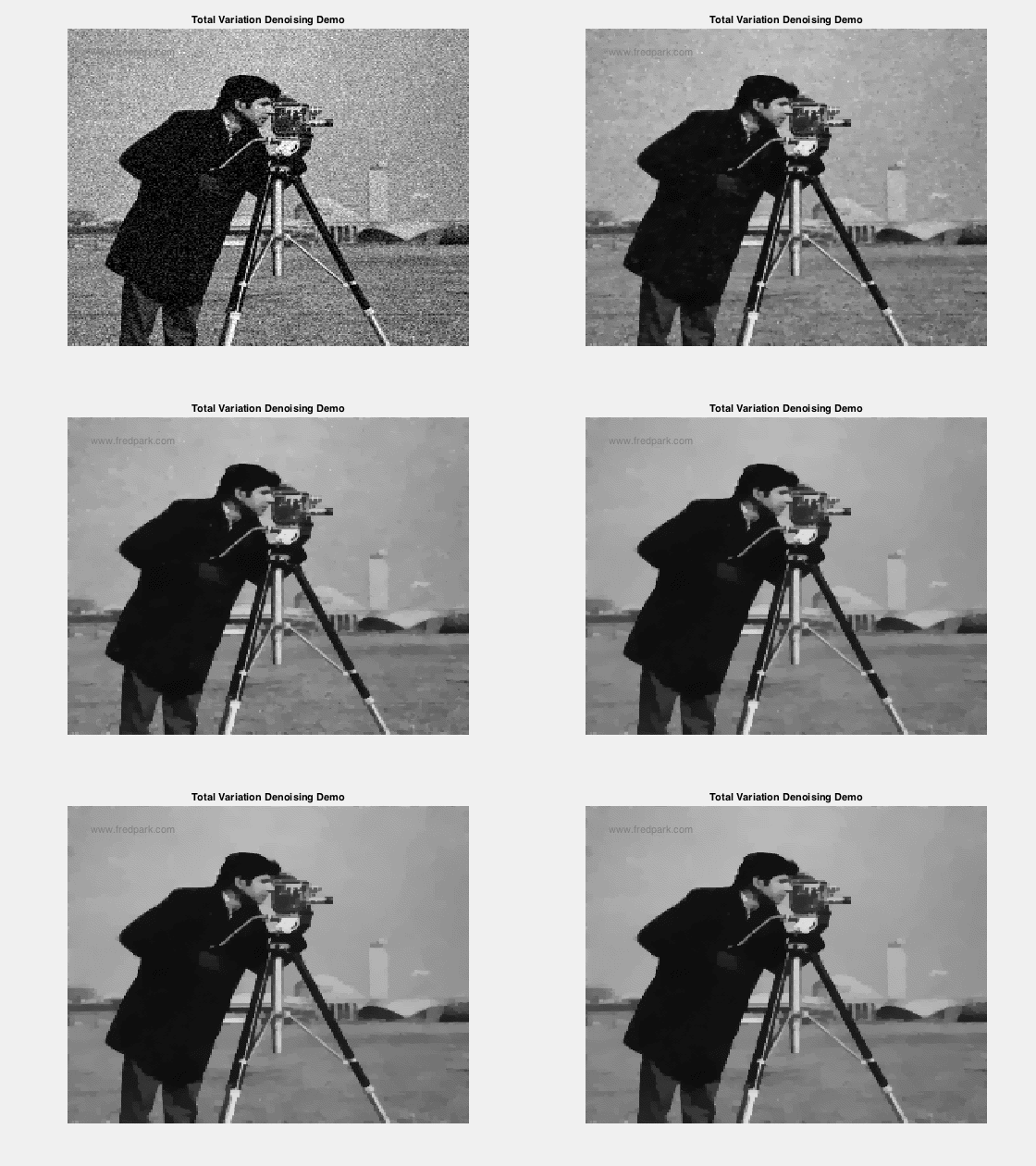
where $\nabla J[u]$ denotes the functional gradient (more on this in later blog posts!). Intermediate results for increasing values of $t$ from the gradient descent to minimize the TV model are observed below. Note how the noise is removed as the iterates approach a minimum of the functional $J[u]$.
Picture
4 Comments
Pool Installation New Haven link
6/30/2022 08:11:52 pm

Lovvely blog you have here

Reply
H
7/12/2022 10:06:34 pm

Prof. Park, This is a bit late....Thank you for the excellent explanation of the ROF method. You mention, "...where ∇J[u] denotes the functional gradient (more on this in later blog posts!)...". Can you please point to the corresponding blogs in which the functional gradient is discussed? Thanks.

Reply
Fredrick Park link
7/13/2022 09:49:37 am

Hi H, thank you for the comment.
Peter Olver has a nice explanation of the functional gradient on pages 11-14 (top of page pg. 14)
see: https://www-users.cse.umn.edu/~olver/ln_/cvc.pdf

I plan on updating the blog later this summer with more detailed explanations along with some interesting work on neural network sparsification (machine learning).

Reply
H W
7/14/2022 08:36:25 am

Prof. Park, Thank you very much for your reply. I will study Prof. Olver's notes. I look forward to your blogs. Regards, H W


Leave a Reply.

    Fred Park

    Assistant Professor at Whittier College.
    Applied Mathematician
    working in Mathematical Image Processing, Computer Vision, and Machine Learning.

    Archives

    October 2020
    May 2018
    April 2018
    November 2016
    September 2016
    May 2016
    April 2016
    February 2016
    December 2015

    Categories

    All

    RSS Feed

Links:
Whittier College
Whittier College Math 
UCLA Math
UCI Applied Math