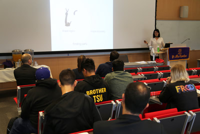
The 2018 Pi Mu Epsilon Math Honor Society induction and talk was wonderful. A big thank you to our invited speaker Professor Kathryn Leonard! Congratulations to all the new inductees! See you all at the next PME event in 2019!

Happy start of the Fall semester! We are now in the newly renovated Science and Learning Center (SLC) which was a $50 million dollar state of the art renovation. 

In our Pi Mu Epsilon Talk last week, Dr. Weisbart talked about the noise process and how noise manifests itself in images. Here I say a few words about the image denoising process, i.e. noise removal. Given a grayscale image $f:[0,1]\times[0,1]\rightarrow [0,255]$ where $f(x,y)=0$ denotes black and $f(x,y)=255$ denotes white; any value in between is a shade of gray. Color images are the extension where a pixel location $(x,y)$ maps to a vector $[R,G,B]$. Each component $R$, $G$, and $B$ are grayscale images themselves representing the red, green, and blue channels respectively. In the talk last week, the speaker spoke about Poisson noise processes. In general, since such noise processes can be approximated by Gaussian noise via the Central Limit Theorem, we assume an additive Gaussian noise from a modeling perspective. i.e. if $u_c$ denotes the clean image, then the image $f$ degraded by noise is modeled as the following:
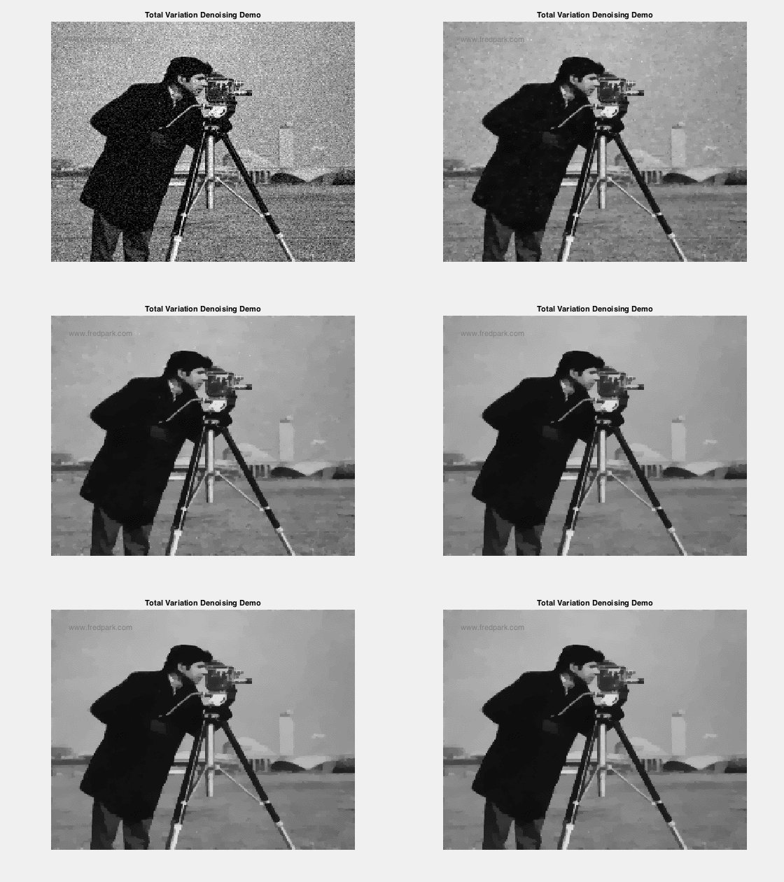
$$f(x,y) =  u_c(x,y) + \eta(x,y)$$
where $\eta(x,y)$ is a random variable from a Gaussian distribution of mean zero and standard deviation $\sigma$. Thus, the image denoising problem is the inverse problem of finding $u_c$ given the noisy image $f$ and some statistics on the noise.

One of the most celebrated and utilized image denoising models is the TV-Denoising Model from Rudin, Osher, and Fatemi. The model is in a functional minimization form:
$$\min_{u} \left\{ J[u] =  \frac{1}{2}\int_{\Omega} (f-u)^2\,dx + \lambda \int_{\Omega} |\nabla u| \right\}$$
where $\Omega$ is the image domain (rectangle) and the Total variation semi-norm $\int |\nabla u|$ is defined in the distributional sense:
$$TV(u) = \int_{\Omega}|\nabla u| = \sup \left\{\int_{\Omega} u(x) \xi(x) \, dx \, | \, \xi \in C_c^1(\Omega, \mathbf{R}^n), \ \|\xi\|_{\infty} \leq 1\right\}.$$ 
The model is a balance between data fitting and regularity where the parameter $\lambda$ controls this tradeoff.

There are numerous ways to minimize the above TV model but one of the simplest is via gradient descent:
$$u_ t = -\nabla J[u] = f-u + \nabla \cdot \frac{\nabla u}{|\nabla u|}$$
where $\nabla J[u]$ denotes the functional gradient (more on this in later blog posts!). Intermediate results for increasing values of $t$ from the gradient descent to minimize the TV model are observed below. Note how the noise is removed as the iterates approach a minimum of the functional $J[u]$.

Photo of our new inductees along with our guest speaker and returning members of Pi Mu Epsilon. All in all a great time! Congrats to our new members!

Lots of fun conversations and stories at dinner as well. Looking forward to next year!

Here's a photo from last year's induction ceremony and talk (2015). Our invited speaker was Alice Silverberg from UCI. 

In Calculus I (Math 141A) we are learning Newton's Method. It all starts with a simple linear approximation to a function and seeing where the approximation crosses the x-axis. That crossing point yields a new starting point for another linear approximation and an iterative scheme is created.

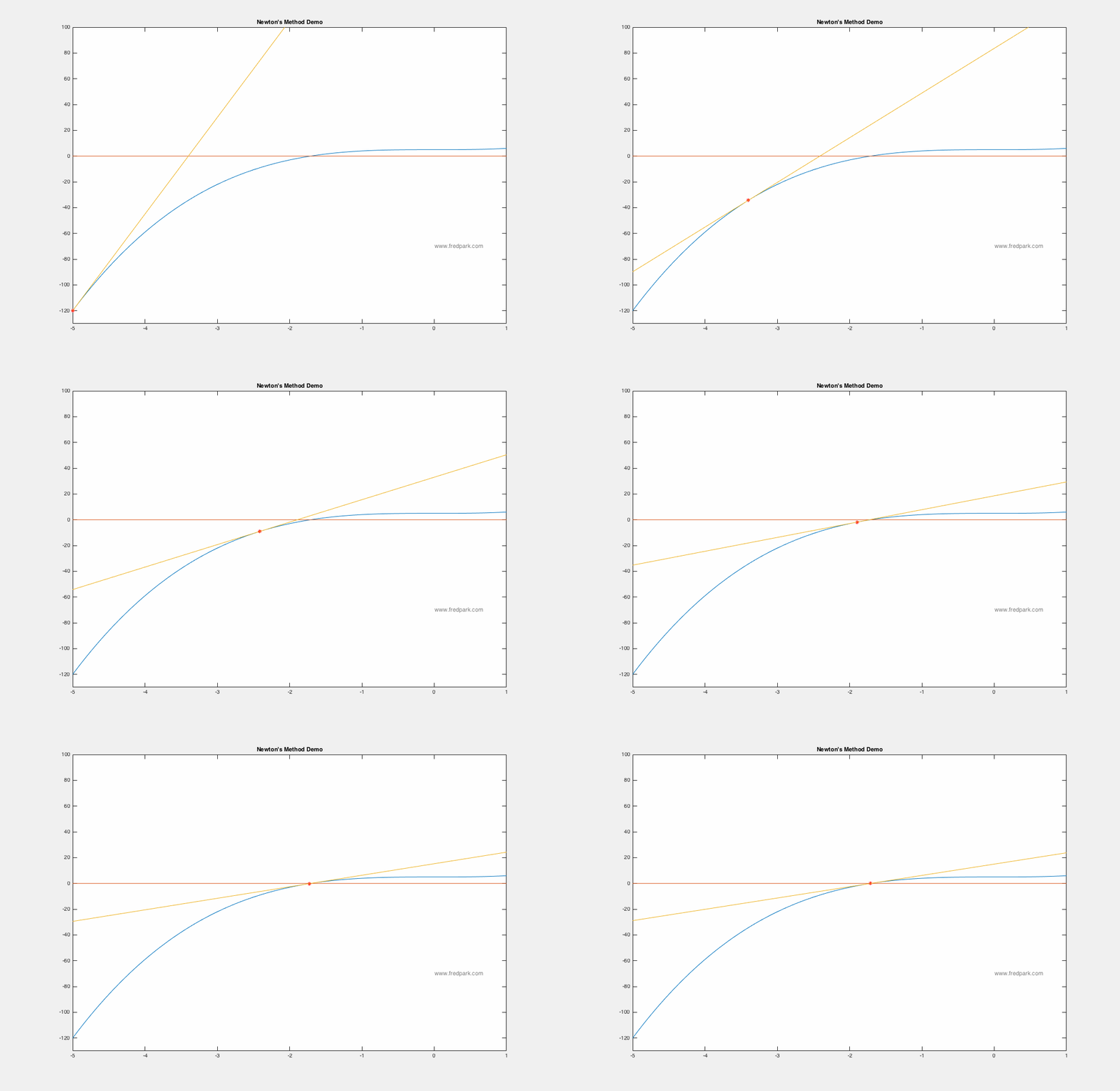
$$x_{n+1} = x_n - \frac{f(x_n)}{f'(x_n)}.$$

Newton's method applied to the function $f(x) = x^3 + 5$ is seen below using the starting point $x_0 = -5$. Within 7 iterations, $|f(x_7)|<10^{-15}$.

In my Math Modeling course last Fall 2015, we studied an optimization algorithm known as gradient descent. The main application is to find minimizers of functions or functionals. More on the latter later. 

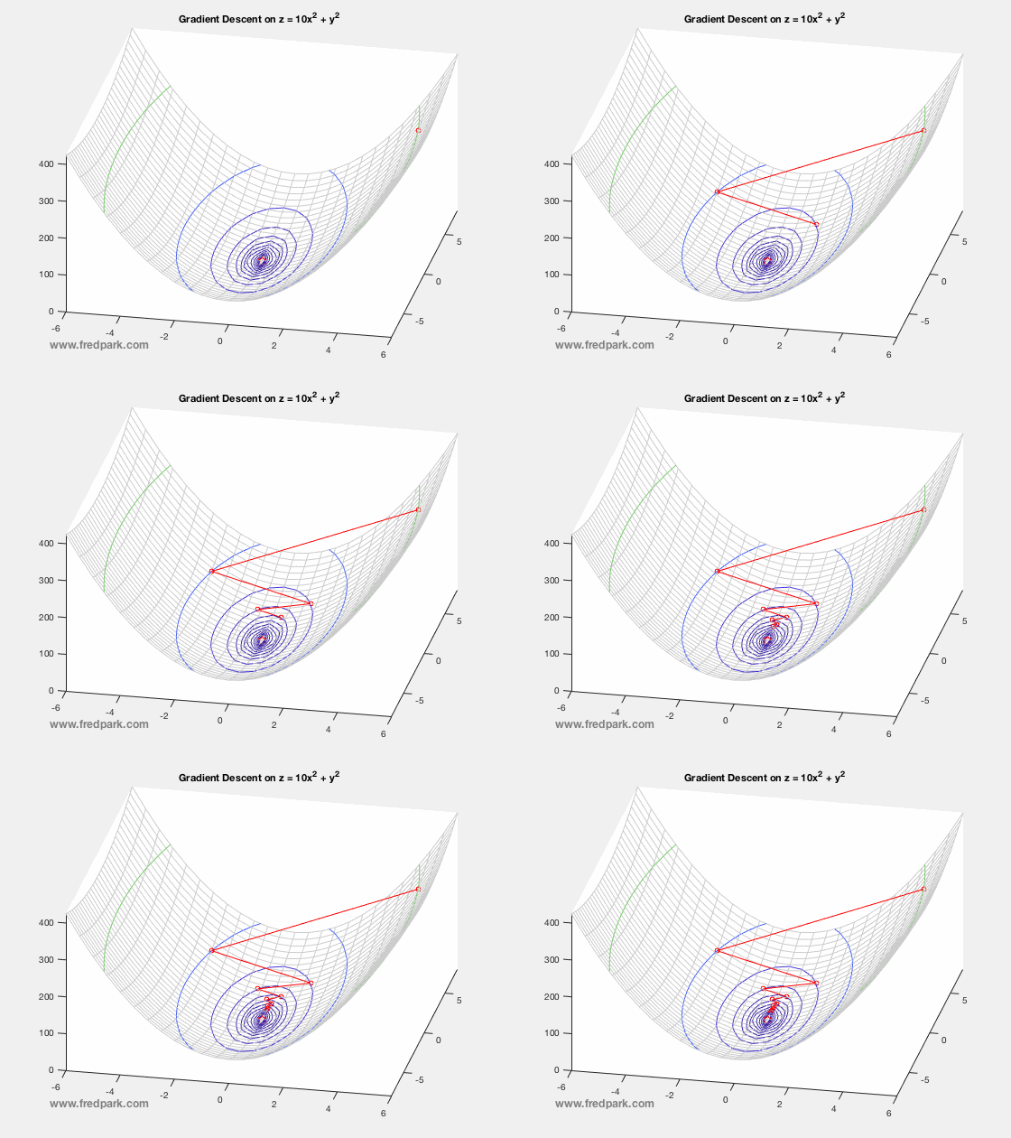
Let $F(\mathbf{x})$ be a function defined and differentiable on some domain $\Omega \subseteq \mathbb{R}^n$. Then, gradient descent is the following iterative scheme:
$$
\mathbf{x}^{n+1} = \mathbf{x}^n -\delta \nabla F(\mathbf{x}^n) \ \ \ (1)
$$
where $\, \delta$ is a time-step parameter and $\, \nabla F(\mathbf{x})$ denotes the gradient of $\, F$. From multi-variable calculus, we know that for a function of 2 variables $z=F(x,y)$ with graph in $\mathbb{R}^3$, the gradient vector points in the direction of steepest ascent of the function $\, F$. Thus, $-\nabla F$ points in the steepest descent direction. This is the key premise of gradient descent. The method is local in nature and for a sufficiently well behaved function ($\nabla F$ Lipschitz continuous), will always move towards a minima from the point obtained from the previous iteration. Thus, it will always converge in that case. Notable caveats include slow convergence near minima, linear convergence rate at best, and non-optimal convergence if the Hessian Matrix is ill-conditioned. An example of slow convergence due to a zig-zagging phenomenon is observed below.